Analysis & Implementation of Mandelbrot Sets and Julia Fractals on Raspberry Pi3 using IPython

I. CONVERGENCE, DIVERGENCE, CHAOS
To begin with, let us consider a Function, which multiplies by 2. We can see that starting with some initial or seed value greater than 0, say 2, and repeatedly applying this function, “Multiply by 2” results in values which grow not only just steadily but at an accelerated rate, growing even faster. We then say that this function is divergent and diverges to higher values. Let us look at the graph of this function.

Now, consider the function “divide by 3” with initial value or seed value greater than 0, say 10. We see that successive values get smaller and smaller. We can see the values get closer and closer to zero, but never reach it. We say this function converges towards zero. Thus, the function “divide by 3” is convergent.

Now let us combine both these together and have a function like, “multiply by -0.8” and when we apply it successively we get something quite interesting and dynamic. When we see the graph it looks something like,

The values toggle between positive and negative values, as you would expect if you successively multiplied by a negative number. This behavior which reflects some of the more interesting things we might see in nature, such as the decay of a pendulum swing or the vibrations of a plucked guitar string fading away.
Now, let’s look at an iterative function,

which was developed by scientists trying to model population growth. It’s called the Logistic Map, but the name doesn’t really explain much so let’s not worry about it. The following diagram shows this function.

Now this function depends on two values, one is the value of ‘r’ and the other is the value of x. For different values of ‘r’ we can consider some value of x and apply it successively to this function. And to avoid any doubt, let’s explain what we mean by successively. We start with x, say as 0.2 and r =1. Then r.x.(1-x) is 1 * 0.2 * (0.8) = 0.16 which is the output value. This value is then put back into the function as input for the next iteration which gives 0.1344, and so on successively.
Let us try again, but this time with r set as 2 instead of 1.The Graph looks something like this now,

Now, this looks interesting. With r=1, the values were converging towards 0, and now with r=2, the values are converging towards 0.5. Similarly, if we try with r=3, we see the following graph,
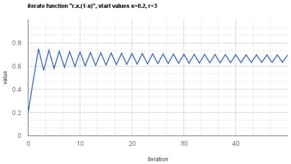
The same function, has now given us behavior which oscillates, like the periodic oscillating function we saw earlier. Again, we didn’t change the function to get this very different behavior, we simply modified the value of one of its parameters.Now, let us see what happens for r=4, for which we get a Graph like this,

The behavior that we can see appears unpredictable, unruly & random. There is no observable pattern here like a gentle convergence, or even a rapid divergence, and not even something we can pick out as a regular periodic oscillation. What we have found here, is Chaos. So, now our Map of Functions looks something like this,

II. COMPLEX FUNCTIONS
The difference between this function from previous functions is Complex Functions work on Complex Numbers, instead of on natural numbers. Let us take this function,

where, z and c are complex numbers.
Any complex number consists of two parts, the Real part and the Imaginary part. Let us take z as (a+bi) ,where a is the Real part and b is the Imaginary part. On expanding we get,

Now, let us try out this function with some examples. Let us set z= (0+0i) and c=(2+2i).
Function: z^2 + c, for complex z & c.
Let seed z=(0+0i), c set to (2 + 2i)
Iteration Real Imaginary Magnitude
0 0 0 0
1 2 2 2.8284
2 2 10 10.1980
3 -94 42 102.9563
4 7074 -7894 10599.8449


Let seed z=(0+0i), c set to (2 + 2i)
Iteration Real Imaginary Magnitude
0 0 0 0
1 2 2 2.8284
2 2 10 10.1980
3 -94 42 102.9563
4 7074 -7894 10599.8449
In the first iteration with z set to 0+0i and c=(2+2i), and
applying to the function we get 2+2i.
In the next iteration we apply this value as, z and c=(2+2i) and next
we get 2+10i. On plotting the
Magnitude value w.r.t the number of iterations we get,
The graph shows that the magnitude values are getting larger and larger with the increasing number of iterations. Thus for z=0+0i, the values are diverging.
Similarly, if we set c=(0.4+0.4i), we will get the following values and on entering them like the previous table,
Function: z^2 + c, for complex z & c.
Let seed z=(0+0i), c set to (0.4 + 0.4i)
Iteration Real Imaginary Magnitude
0 0 0 0
1 0.4 0.4 0.565685
2 0.4 0.72 0.823650
3 0.416 0.976 0.976886
4 -0.5508 0.4812032 0.731428
5 0.471874 -0.13013717 0.489490
6 0.6057295 0.277183252 0.666137
From, the graph we can see that the magnitude values are growing but not at a fast rapid rate like before.
Similarly, if we set c=(-0.3+0.4i) and plot the Magnitude values we get,

The Magnitude values oscillate before settling down and approaching 0.3819.
Similarly, if we set c=(0.3+0.4i) and plot the Magnitude values we get,

From the graph, the magnitude values neither converge nor diverge but simply oscillate.
The boundary between c=0.3+0.4i and the c=-0.3+0.4i is quite interesting. It throws up two very interesting Magnitude plots. Hence, now we will consider somewhere around this boundary, so we will first, vary the Real part by 0.01 for which we set, c=0.33+0.577i, c=0.34+0.577i and c=0.32+0.577i and plot the Magnitude Graph plots for z=0+0i.

For, c=0.32+0.577i ,we get,

For, c=0.33+0.577i ,we get,

For, c=0.34+0.577i, we get,

From, this we can see that close to c=0.33+0.577i, the behavior of the Magnitude plot changes drastically.
Similarly now, we will vary the Imaginary part by 0.01 for which we set, c=0.33+0.587i & c=0.33+0.567i and plot the Magnitude Graph plots for z=0+0i.
For, c=0.33+0.587i, we get,

For, c=0.33+0.567i, we get,

To summarize, we can see the Divergence Map based on the different values of c, as covered now,

Based on the above results and our understanding, we can now define a Mandelbrot Set.
Basically Mandelbrot Set is a set of Complex Numbers for which the function,

does not diverge. Mandelbrot set images can be created by having a set of complex numbers and determining, for each sample point c, if the result of iterating the above function, the magnitude diverges or not.
III. IMPLEMENTATION OF MANDELBROT SET ON RASPBERRY PI3
This part provides the Implementation
of Mandelbrot Sets and Julia Fractals on RaspberryPi using IPython’s SciPy.
First, check if Python is
installed or not.
#python –version
The version we have used is Python
Version 2.7.12. Next we see how to install SciPy and other associated Python
packages.
To install via pip on Mac or
Linux, first upgrade pip to the latest version:
#python -m pip
install --upgrade pip
Then install the SciPy stack
packages with pip. We recommend a user install, using the --user flag to pip
(note: don’t use sudo pip, that will give problems). This installs packages for
your local user, and does not need extra permissions to write to the system
directories:
#pip install --user numpy scipy matplotlib
ipython jupyter pandas sympy nose
For user installs, make sure your user
install executable directory is on your PATH. Here are example commands for
setting the user PATH:
LINUX:
# Consider adding this at the end
of your ~/.bashrc file
# export
PATH="$PATH:/home/your_user/.local/bin"
OSX:
# Consider adding this at the end
of your ~/.bash_profile file
# export PATH="$PATH:/Users/your_user/Library/Python/3.5/bin"
If installing without using pip,
then please use the below command,
UBUNTU & DEBIAN:
# sudo apt-get install
python-numpy python-scipy python-matplotlib ipython ipython-notebook
python-pandas python-sympy python-nose
Once we are through this part, let us start our design,
Open the Python Terminal and first import this Python Magic function, %pylab,
%pylab
import scipy.ndimage
Later we will see, how we are using scipy.ndimage during drawing the plots. Now, let us first define a Python routine, mandel, which will take two input parameters
def mandel(c, maxiter):
z = complex(0, 0)
for iteration in range(maxiter):
z = (z*z) + c
if abs(z) > 4:
break
pass
pass
return iteration
Now, the above routine is the kernel which takes the chosen point represented by complex c, and returns the number of iterations taken to cross a threshold on its way to divergence. The mandel routine takes the parameter c, the complex number representing the point to be tested for divergence. The routine returns the number of iterations it took to cross the threshold.
What if the point doesn’t diverge and has a nice tight orbit? Will we keep running the iterations forever because the threshold would never be crossed ? Well if we did that we’d never progress beyond that single point being tested, and eventually our code would fail as it would run out of space to keep track of the iterations. We need a way of stopping the calculations when we are satisfied that the point won’t diverge. A good enough way, is to define the maximum number of iterations the routine is to be applied. It must be large enough to convince us that the point won’t diverge. This is guaranteed by the maxiter parameter.
If we keep few iterations, then the finer details, when plotted, are not sufficiently defined. Two points which are close to each other may appear like they don’t diverge, but with more iterations it may become apparent that one does and the other doesn’t. This distinction defines the detail that is uncovered and plotted. Thus increase the number of Iterations and the details become more finer. But a large value of Iteration shall make the calculations take more time.
Hence a Trade-off !
x_list = linspace(-2.25, 0.75, 1000)
y_list = linspace(-1.5, 1.5, 1000)
x_len = len(x_list)
y_len = len(y_list)
atlas = empty((x_len, y_len))
for ix in range(x_len):
for iy in range(y_len):
cx = x_list[ix]
cy = y_list[iy]
c = complex(cx, cy)
atlas[ix, iy] = mandel(c, 40)
pass
pass
Next, we will see how to use this routine mandel. We will define two arrays elements which will hold a series of equally spaced values for X-axis and Y-axis which will together represent a complex number. The series elements x_list and y_list are holding 1000 elements each from -2.25 to 0.75 along the X-Axis and -1.5 to 1.5 along the Y-Axis. We create an empty series element, atlas which should be able to hold a maximum number of elements, owing to condition, if all the elements do not diverge, hence we shall keep it as two-dimensional of size (x_len * y_len). Now, we will iterate along for two variables ix and iy, where iy will vary from 0 to y_len for each value ix varying from 0 to x_len.
Next, we pick each corresponding X-axis values and Y-axis values and assign them to the complex, c and pass them over to our routine, mandel with maxiter set to 40. This completes the values that we are now able to collect to plot our Mandelbrot set.
Now, we will look at the interesting part of plotting them. We will now simply call imshow to display our Mandelbrot Set. The atlas.T tells the imshow routine to consider the Transpose of the two dimensional array, atlas. The Interpolation that we have considered here is Lanczos, one can consider Nearest neighbor, Bi-Linear, Bi-Cubic, Spline, Gaussian et al to observe upon.
imshow(smoothed_atlas, interpolation="lanczos")
This would display our Mandelbrot
Set as follows,

Now, let us make it a little bit more interesting. Let us try with different image processing DSP Filters and see for ourselves the results of our observation. Let us first, try with a Gaussian Filter kernel, which is a kind of Low-Pass, Smoothing filter.
smoothed_atlas = scipy.ndimage.gaussian_filter(atlas.T, 2)
imshow(smoothed_atlas, interpolation="lanczos")
This would display our Mandelbrot as follows,

Clearly, the edges of our Mandelbrot Set look smoothed now.
Now, lets try some Gradient filtering on our Mandelbrot, using a Laplacian kernel.
smoothed_atlas = scipy.ndimage.gaussian_filter(atlas.T, 2)
scipy.ndimage.laplace(atlas.T, smoothed_atlas, 'mirror', 20.0)
imshow(smoothed_atlas, interpolation="lanczos")
This would display our Mandelbrot as follows,

Similarly, using a Sobel Kernel,
smoothed_atlas = scipy.ndimage.gaussian_filter(atlas.T, 2)
scipy.ndimage.sobel(atlas.T, 1, smoothed_atlas, 'mirror', 0.0)
imshow(smoothed_atlas, interpolation="lanczos")
This would display our Mandelbrot as follows,

Similarly, using a Prewitt Kernel,
smoothed_atlas = scipy.ndimage.gaussian_filter(atlas.T, 2)
scipy.ndimage.prewitt(atlas.T, 1, smoothed_atlas, 'mirror', 20.0)
imshow(smoothed_atlas, interpolation="lanczos")
would display our Mandelbrot as follows,

IV. JULIA SETS
There is very subtle difference from Mandelbrot Set.
In case of Mandelbrot Set we saw that we chose a Rectangle in the Complex plane
marked by evenly spaced points in the X-axis and Y-axis and applied the function,
z^2+c , in an iterative way on each of those points, where c was the point being tested,
resulted in the orbit escaping and diverging, or not. And if it does, we color the point
according to how fast the point diverges.
The difference is that the roles of z and c are reversed. Instead of c representing the
point being tested, in Mandelbrot, it is now kept constant and z is varied.
That’s it. That is the only difference. This simple diagram illustrates the same,

The following shows the calculating kernel routine, Julia(z, c, maxiter) based on Mandel(c, maxiter) we wrote earlier,
def julia(z, c, maxiter):
for iteration in range(maxiter):
z = (z*z) + c
if abs(z) > 4:
break
pass
pass
return iteration
Clearly, we can see that z is not fixed now, but is passed as a parameter, but c is constant and is passed to the routine. Let us see how,
x_list = linspace(-2, 2, 1000)
y_list = linspace(-2, 2, 1000)
y_len = len(y_list)
x_len = len(x_list)
c = complex(-0.35, 0.65)
atlas = empty((x_len, y_len))
for ix in range(x_len):
for iy in range(y_len):
cx = x_list[ix]
cy = y_list[iy]
z = complex(cx, cy)
atlas[ix, iy] = julia(z, c, 80)
pass
pass
imshow(atlas.T, interpolation="lanczos")
Thus, we get our Julia set,

Now, let us make it more interesting by using Image Processing DSP Filters on our Output, let us apply some Gaussian filtering,
smoothed_atlas = scipy.ndimage.gaussian_filter(atlas.T, 2)
scipy.ndimage.fourier_gaussian(atlas.T, 0.5, -1, 1, smoothed_atlas)
imshow(smoothed_atlas, interpolation="lanczos")
which displays the following,

Now, let us change the c value and z values. Let us set c= -0.768662 + 0.130477i and z as follows,
c = complex(-0.768662, 0.130477)
x_list = linspace(-1, 1, 1000)
y_list = linspace(-1, 1, 1000)
On plotting using Gaussian we get,
smoothed_atlas = scipy.ndimage.gaussian_filter(atlas.T, 2)
imshow(smoothed_atlas, interpolation="lanczos")

On applying Fourier Gaussian filter, we get,
scipy.ndimage.fourier_gaussian(atlas.T, 0.5, -1, 1, smoothed_atlas)
imshow(smoothed_atlas, interpolation="lanczos")

On, applying some gradient filters like Laplacian, we get,
scipy.ndimage.laplace(atlas.T, smoothed_atlas, 'mirror', 20.0)
imshow(smoothed_atlas, interpolation="lanczos")

V. SOME EXERCISES
And, here are a few teasers, which are produced by the some ways. Readers can try their hands in generating the same,

Same with, Mandelbrot too,

And our Classic Mandelbrot,

And our Classic Julia too,

Isn’t it a beauty, how simple looking functions can produce such exquisite detail.
VI. EPILOGUE
This completes our journey of the Mandelbrot Sets & Julia Fractals.
Users are free to experiment with different parameters like c, z and maxiterations. Here are few snapshots of my Implementation on Raspberry Pi 2. Hope I am able to inspire people into trying out something on Mathematics which they can feel and relate themselves too, instead of solving equations and derivations.
This primer should help Teachers & Educationists to show how Mathematics can be interesting in Real world, how from the world of equations, something can be turned out by modifying a few parameters & some basic mathematical stuff. I hope people understand my aim and try something along those lines.

VII. REFERENCES
1. https://commons.wikimedia.org/wiki/Mandelbrot_set
2. http://math.wikia.com/wiki/Mandelbrot_Set
3. https://rosettacode.org/wiki/Mandelbrot_set
4. http://yozh.org/mset_index/ - Rhapsody in Numbers
5. http://wiki.c2.com/?MandelbrotSet
VIII. RESOURCES
This completes our journey of the Mandelbrot Sets & Julia Fractals.
Below are the sources for Mandelbrot & Julia Fractals. Enjoy & show me further new designs as we keep experimenting.
# MandelBrot
%pylab
import scipy.ndimage
def mandel(c, maxiter): z = complex(0, 0)
for iteration in range(maxiter):
z = (z*z) + c
if abs(z) > 4:
break
pass
pass
return iteration
x_list = linspace(-2.25, 0.75, 1000)
y_list = linspace(-1.5, 1.5, 1000)
x_len = len(x_list)
y_len = len(y_list)
atlas = empty((x_len, y_len))
for ix in range(x_len):
for iy in range(y_len):
cx = x_list[ix]
cy = y_list[iy]
c = complex(cx, cy)
atlas[ix, iy] = mandel(c, 40)
pass
pass
smoothed_atlas = scipy.ndimage.gaussian_filter(atlas.T, 2)
scipy.ndimage.fourier_gaussian(atlas.T, 1.5, -1, 1, smoothed_atlas)
imshow(smoothed_atlas, interpolation="lanczos")
# Julia Fractals
%pylab
import scipy.ndimage
def julia(z, c, maxiter):
for iteration in range(maxiter):
z = (z*z) + c
if abs(z) > 4:
break
pass
pass
return iteration
x_list = linspace(-2, 2, 1000)
y_list = linspace(-2, 2, 1000)
y_len = len(y_list)
x_len = len(x_list)
c = complex(-0.35, 0.65)
atlas = empty((x_len, y_len))
for ix in range(x_len):
for iy in range(y_len):
cx = x_list[ix]
cy = y_list[iy]
z = complex(cx, cy)
atlas[ix, iy] = julia(z, c, 80)
pass
pass
imshow(atlas.T, interpolation="lanczos")
smoothed_atlas = scipy.ndimage.gaussian_filter(atlas.T, 2)
scipy.ndimage.laplace(atlas.T, smoothed_atlas, 'mirror', 20.0)
scipy.ndimage.fourier_gaussian(atlas.T, 0.5, -1, 1, smoothed_atlas)
imshow(smoothed_atlas, interpolation="lanczos")
With Regards,
Thank You,
Rajiv.
No comments:
Post a Comment